43 excel how to add data labels to all series
Add a DATA LABEL to ONE POINT on a chart in Excel Steps shown in the video above: Click on the chart line to add the data point to. All the data points will be highlighted. Click again on the single point that you want to add a data label to. Right-click and select ' Add data label ' This is the key step! Right-click again on the data point itself (not the label) and select ' Format data label '. Create Dynamic Chart Data Labels with Slicers - Excel Campus Step 6: Setup the Pivot Table and Slicer. The final step is to make the data labels interactive. We do this with a pivot table and slicer. The source data for the pivot table is the Table on the left side in the image below. This table contains the three options for the different data labels.
excel - Change format of all data labels of a single series at once ... Go to the chart and left mouse click on the 'data series' you want to edit. Click anywhere in formula bar above. Don't change anything. Click the 'tick icon' just to the left of the formula bar. Go straight back to the same data series and right mouse click, and choose add data labels This has worked in Excel 2016.

Excel how to add data labels to all series
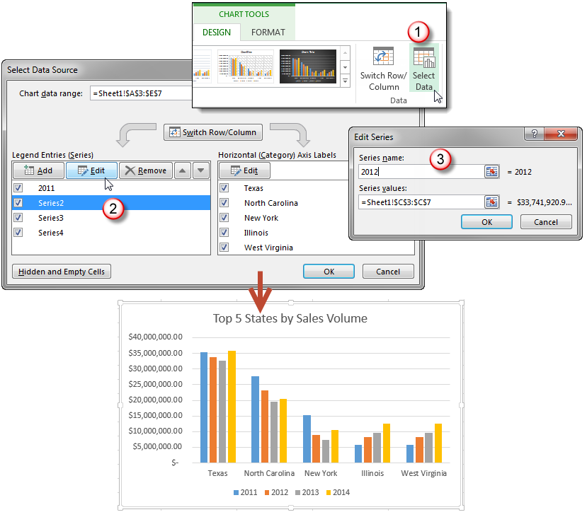
How to Rename a Data Series in Microsoft Excel - How-To Geek To begin renaming your data series, select one from the list and then click the "Edit" button. In the "Edit Series" box, you can begin to rename your data series labels. By default, Excel will use the column or row label, using the cell reference to determine this. Replace the cell reference with a static name of your choice. How To Add Data Labels In Excel - die1.info You can now configure the label as required — select the content of. To format data labels in excel, choose the set of data labels to format. After picking the series, click the data point you want to label. To Format Data Labels In Excel, Choose The Set Of Data Labels To Format. Secondly, click on the chart elements option and press axis titles. Bubble Chart in Excel - Step-by-step Guide Select the "Sales" series, right-click, and choose "Add Labels". You will see only zeros, but no worry! Right-click on the labels; the "Format Data Labels" will appear. Under the "Label Options", check the "Values From Cells" checkbox. Select the B3:B25 range. Finally, set the label position to "Center". Last but not ...
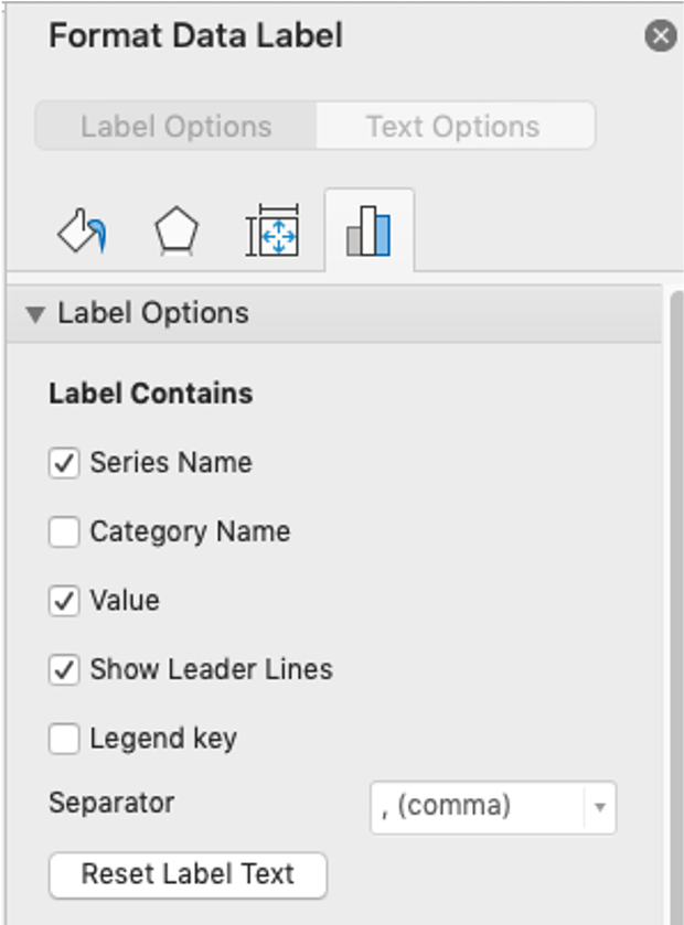
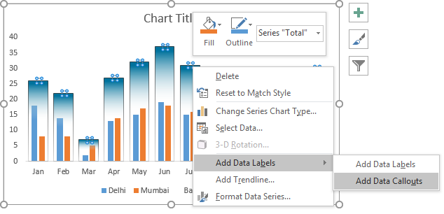
Excel how to add data labels to all series. Series.ApplyDataLabels method (Excel) | Microsoft Docs For the Chart and Series objects, True if the series has leader lines. ShowSeriesName: Optional: Variant: Pass a Boolean value to enable or disable the series name for the data label. ShowCategoryName: Optional: Variant: Pass a Boolean value to enable or disable the category name for the data label. ShowValue: Optional: Variant Add or remove data labels in a chart - support.microsoft.com Click the data series or chart. To label one data point, after clicking the series, click that data point. In the upper right corner, next to the chart, click Add Chart Element > Data Labels. To change the location, click the arrow, and choose an option. If you want to show your data label inside a text bubble shape, click Data Callout. Adding Data Labels to Your Chart (Microsoft Excel) - ExcelTips (ribbon) Make sure the Design tab of the ribbon is displayed. (This will appear when the chart is selected.) Click the Add Chart Element drop-down list. Select the Data Labels tool. Excel displays a number of options that control where your data labels are positioned. Select the position that best fits where you want your labels to appear. Dynamically Label Excel Chart Series Lines - My Online Training Hub Step 1: Duplicate the Series. The first trick here is that we have 2 series for each region; one for the line and one for the label, as you can see in the table below: Select columns B:J and insert a line chart (do not include column A). To modify the axis so the Year and Month labels are nested; right-click the chart > Select Data > Edit the ...
Add data labels excel - wapnj.atbeauty.info To add data to the chart: Scroll down to the end of the existing data and input the new labels and data into the first blank rows: If necessary, use Edit/Copy and Edit/Paste to copy any formulas down to the new rows. Next, click on the chart to view the QI Macros chart menu. This menu is sometimes hard to find in the Excel 2013-2019 and Office. How to Change Excel Chart Data Labels to Custom Values? - Chandoo.org First add data labels to the chart (Layout Ribbon > Data Labels) Define the new data label values in a bunch of cells, like this: Now, click on any data label. This will select "all" data labels. Now click once again. At this point excel will select only one data label. How to Add Labels to Show Totals in Stacked Column Charts in Excel Press the Ok button to close the Change Chart Type dialog box. The chart should look like this: 8. In the chart, right-click the "Total" series and then, on the shortcut menu, select Add Data Labels. 9. Next, select the labels and then, in the Format Data Labels pane, under Label Options, set the Label Position to Above. 10. Adding rich data labels to charts in Excel 2013 | Microsoft 365 Blog Once the series is selected, I can right-click any column to pull up the context menu, then click the Add Data Labels entry. When I click Add Data Labels, I get the following result. To reposition any single data label, all I have to do is double-click the data label I want to move, then drag it to the desired position on the chart.
Excel Charts: Dynamic Label positioning of line series - XelPlus Select your chart and go to the Format tab, click on the drop-down menu at the upper left-hand portion and select Series "Actual". Go to Layout tab, select Data Labels > Right. Right mouse click on the data label displayed on the chart. Select Format Data Labels. Under the Label Options, show the Series Name and untick the Value. Excel chart changing all data labels from value to series name ... By selecting chart then from layout->data labels->more data labels options ->label options ->label contains-> (select)series name, I can only get one series name replacing its respective label values. For more than hundred series stacked in columns i want them all to be changed at once, is there any way out? why it does not change them all at once? How to set all data labels with Series Name at once in an Excel 2010 ... chart series data labels are set one series at a time. If you don't want to do it manually, you can use VBA. Something along the lines of Sub setDataLabels () ' ' sets data labels in all charts ' Dim sr As Series Dim cht As ChartObject ' With ActiveSheet For Each cht In .ChartObjects For Each sr In cht.Chart.SeriesCollection sr.ApplyDataLabels Change the format of data labels in a chart Tip: Make sure that only one data label is selected, and then to quickly apply custom data label formatting to the other data points in the series, click Label Options > Data Label Series > Clone Current Label. Here are step-by-step instructions for the some of the most popular things you can do.
Adding rich data labels to charts in Excel 2013 | Microsoft ...
Excel Chart - Selecting and updating ALL data labels Dim objSeries As Series ActiveSheet.ChartObjects ("Chart 2").Activate With ActiveChart For Each objSeries In .SeriesCollection With objSeries .Format.Line.Transparency = 0 .Format.Line.Weight = 0.1 .Format.Line.ForeColor.RGB = 1 End With objSeries.DataLabels.Select Selection.ShowSeriesName = True Selection.ShowValue = False Next End With End Sub

Total of chart series – Excel kitchenette
How to set multiple series labels at once - Microsoft Tech Community If the range containing the series names is adjacent to the series values, try the following: Click anywhere in the chart. On the Chart Design tab of the ribbon, in the Data group, click Select Data. Click in the 'Chart data range' box. Select the range containing both the series names and the series values. Click OK.

how to add data labels into Excel graphs — storytelling with data
How to add data labels from different column in an Excel chart? Right click the data series in the chart, and select Add Data Labels > Add Data Labels from the context menu to add data labels. 2. Click any data label to select all data labels, and then click the specified data label to select it only in the chart. 3.

How to Add Data Labels to an Excel 2010 Chart - dummies
Add data labels and callouts to charts in Excel 365 - EasyTweaks.com Step #1: After generating the chart in Excel, right-click anywhere within the chart and select Add labels . Note that you can also select the very handy option of Adding data Callouts. Step #2: When you select the "Add Labels" option, all the different portions of the chart will automatically take on the corresponding values in the table ...

Other Options for Chart Data Labels in PowerPoint 2011 for Mac
Create a multi-level category chart in Excel - ExtendOffice Double click any series in the chart to open the Format Data Series pane. In the pane, change the Gap Width to 0%. 5. Select the spacing1 data series in the chart, go to the Format Data Series pane to configure as follows. 5.1) Click the Fill & Line icon; 5.2) Select No fill in the Fill section. Then these data bars are hidden. 6.

Custom data labels in a chart
Adding series labels - Excel Help Forum Re: Adding series labels Here is a small example. Main data is 200 points. I copied the data set and sorted on x then y values. Only the top 10 points are plotted and have data labels enabled. I used a dynamic named range so changing the value in C1 will alter the number of data labels displayed. Attached Files

Apply Custom Data Labels to Charted Points - Peltier Tech
Excel charts: add title, customize chart axis, legend and data labels Depending on where you want to focus your users' attention, you can add labels to one data series, all the series, or individual data points. Click the data series you want to label. To add a label to one data point, click that data point after selecting the series. Click the Chart Elements button, and select the Data Labels option.
how to add data labels into Excel graphs — storytelling with data
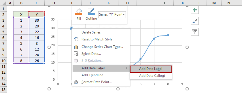
how to add data labels into Excel graphs - storytelling with data You can download the corresponding Excel file to follow along with these steps: Right-click on a point and choose Add Data Label. You can choose any point to add a label—I'm strategically choosing the endpoint because that's where a label would best align with my design. Excel defaults to labeling the numeric value, as shown below.

Directly Labeling Excel Charts - PolicyViz
How to Add Data Labels to an Excel 2010 Chart - dummies If you don't want the data label to be the series value, choose a different option from the Label Options area. You can change the labels to show the Series Name, the Category Name, or the Value. Select Number in the left pane, and then choose a number style for the data labels. Customize any additional options and then click Close.
How to Create a Graph with Multiple Lines in Excel | Pryor ...
How to Add Total Data Labels to the Excel Stacked Bar Chart Step 4: Right click your new line chart and select "Add Data Labels" Step 5: Right click your new data labels and format them so that their label position is "Above"; also make the labels bold and increase the font size. Step 6: Right click the line, select "Format Data Series"; in the Line Color menu, select "No line" Step 7 ...

Change the format of data labels in a chart
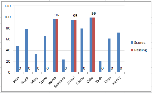
Bubble Chart in Excel - Step-by-step Guide Select the "Sales" series, right-click, and choose "Add Labels". You will see only zeros, but no worry! Right-click on the labels; the "Format Data Labels" will appear. Under the "Label Options", check the "Values From Cells" checkbox. Select the B3:B25 range. Finally, set the label position to "Center". Last but not ...

Dynamically Label Excel Chart Series Lines • My Online ...
How To Add Data Labels In Excel - die1.info You can now configure the label as required — select the content of. To format data labels in excel, choose the set of data labels to format. After picking the series, click the data point you want to label. To Format Data Labels In Excel, Choose The Set Of Data Labels To Format. Secondly, click on the chart elements option and press axis titles.
/Capture-e92aa05671d543ceaf94080eb2687619.JPG)
Understanding Excel Chart Data Series, Data Points, and Data ...
How to Rename a Data Series in Microsoft Excel - How-To Geek To begin renaming your data series, select one from the list and then click the "Edit" button. In the "Edit Series" box, you can begin to rename your data series labels. By default, Excel will use the column or row label, using the cell reference to determine this. Replace the cell reference with a static name of your choice.

424 How to add data label to line chart in Excel 2016

How to Add Total Data Labels to the Excel Stacked Bar Chart ...

Add data labels to your Excel bubble charts | TechRepublic

Add or remove data labels in a chart
How to add data labels from different column in an Excel chart?
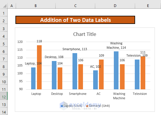
How to Add Two Data Labels in Excel Chart (with Easy Steps ...
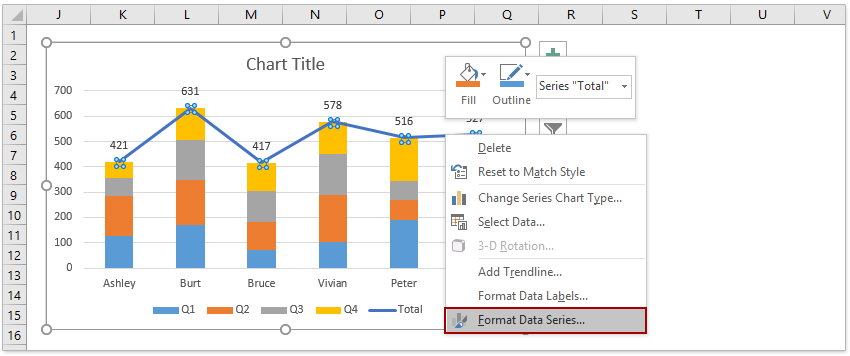
How to add total labels to stacked column chart in Excel?

Adding rich data labels to charts in Excel 2013 | Microsoft ...

How To Show Or Hide Data Labels On MS Excel? | My Windows Hub

Custom Data Labels with Colors and Symbols in Excel Charts ...
How to Create a Graph with Multiple Lines in Excel | Pryor ...

How to set all data labels with Series Name at once in an ...

How to: Display and Format Data Labels | WPF Controls ...
Creative Column Chart that Includes Totals in Excel

How to add data labels from different column in an Excel chart?

How to Use Cell Values for Excel Chart Labels
Add Data Labels Outside End for Dynamic Label Threshold Chart ...

Directly Labeling Your Line Graphs | Depict Data Studio

microsoft excel - Adding data label only to the last value ...

Adding rich data labels to charts in Excel 2013 | Microsoft ...

How to add or move data labels in Excel chart?

Using the CONCAT function to create custom data labels for an ...

How to use data labels in a chart

How to Add Total Data Labels to the Excel Stacked Bar Chart ...

Add Total Values for Stacked Column and Stacked Bar Charts in ...

Apply Custom Data Labels to Charted Points - Peltier Tech

Add or remove data labels in a chart

Excel Charts: Dynamic Label positioning of line series

Change the format of data labels in a chart

How to Customize Your Excel Pivot Chart Data Labels - dummies
Post a Comment for "43 excel how to add data labels to all series"