44 change data labels in excel chart
Add or remove data labels in a chart This displays the Chart Tools, adding the Design, and Format tabs. On the Design tab, in the Chart Layouts group, click Add Chart Element, choose Data Labels, and then click None. Click a data label one time to select all data labels in a data series or two times to select just one data label that you want to delete, and then press DELETE. How to Add Total Data Labels to the Excel Stacked Bar Chart Apr 03, 2013 · Step 4: Right click your new line chart and select “Add Data Labels” Step 5: Right click your new data labels and format them so that their label position is “Above”; also make the labels bold and increase the font size. Step 6: Right click the line, select “Format Data Series”; in the Line Color menu, select “No line”
How to I rotate data labels on a column chart so that they are ... To change the text direction, first of all, please double click on the data label and make sure the data are selected (with a box surrounded like following image). Then on your right panel, the Format Data Labels panel should be opened. Go to Text Options > Text Box > Text direction > Rotate

Change data labels in excel chart
Excel VBA Chart Data Label Font Color in 4 Easy Steps (+ Example) Step 1: Refer to Chart. Refer to the chart with the data label (s) whose font color you want to set. In other words: Create a VBA expression that returns a Chart object representing the applicable chart (with the data label (s) whose font color you want to set). The chart you work with can be either of the following: How to Change Excel Chart Data Labels to Custom Values? - Chandoo.org May 05, 2010 · Now, click on any data label. This will select “all” data labels. Now click once again. At this point excel will select only one data label. Go to Formula bar, press = and point to the cell where the data label for that chart data point is defined. Repeat the process for all other data labels, one after another. See the screencast. Add or remove data labels in a chart - support.microsoft.com Click the data series or chart. To label one data point, after clicking the series, click that data point. In the upper right corner, next to the chart, click Add Chart Element > Data Labels. To change the location, click the arrow, and choose an option. If you want to show your data label inside a text bubble shape, click Data Callout.
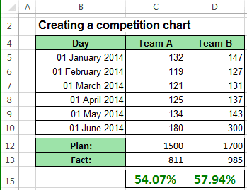
Change data labels in excel chart. Data Labels in Excel Pivot Chart (Detailed Analysis) Next open Format Data Labels by pressing the More options in the Data Labels. Then on the side panel, click on the Value From Cells. Next, in the dialog box, Select D5:D11, and click OK. Right after clicking OK, you will notice that there are percentage signs showing on top of the columns. 4. Changing Appearance of Pivot Chart Labels Is there a way to change the order of Data Labels? Answer Rena Yu MSFT Microsoft Agent | Moderator Replied on April 4, 2018 Hi Keith, I got your meaning. Please try to double click the the part of the label value, and choose the one you want to show to change the order. Thanks, Rena ----------------------- * Beware of scammers posting fake support numbers here. Add or remove data labels in a chart - support.microsoft.com Click the data series or chart. To label one data point, after clicking the series, click that data point. In the upper right corner, next to the chart, click Add Chart Element > Data Labels. To change the location, click the arrow, and choose an option. If you want to show your data label inside a text bubble shape, click Data Callout. Percentage Change Chart – Excel – Automate Excel This tutorial will demonstrate how to create a Percentage Change Chart in all versions of Excel. Percentage Change – Free Template Download Download our free Percentage Template for Excel. Download Now Percentage Change Chart – Excel Starting with your Graph In this example, we’ll start with the graph that shows Revenue for the last 6…
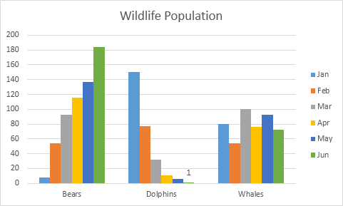
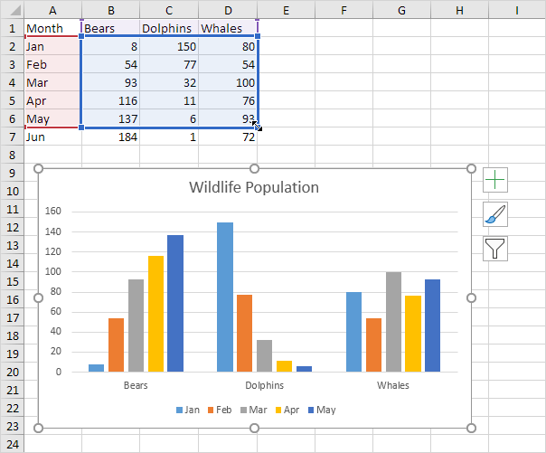
How to add data labels from different column in an Excel chart? Right click the data series in the chart, and select Add Data Labels > Add Data Labels from the context menu to add data labels. 2. Click any data label to select all data labels, and then click the specified data label to select it only in the chart. 3. How to create Custom Data Labels in Excel Charts - Efficiency 365 Create the chart as usual. Add default data labels. Click on each unwanted label (using slow double click) and delete it. Select each item where you want the custom label one at a time. Press F2 to move focus to the Formula editing box. Type the equal to sign. Now click on the cell which contains the appropriate label. Change the format of data labels in a chart To get there, after adding your data labels, select the data label to format, and then click Chart Elements > Data Labels > More Options. To go to the appropriate area, click one of the four icons ( Fill & Line , Effects , Size & Properties ( Layout & Properties in Outlook or Word), or Label Options ) shown here. 1/ Select A1:B7 > Inser your Histo. chart. 2/ Right-click i.e. on the 1st histo. bar (A) > Add Data Labels (numbers are displayed a the top of the bars) 3/ Click one of the numbers that just displayed (the Format Data Labels pane opens on the right) > Check option "Value From Cells" > Select range C2:C7 > OK > Uncheck option "Value".
Edit titles or data labels in a chart - support.microsoft.com The first click selects the data labels for the whole data series, and the second click selects the individual data label. Right-click the data label, and then click Format Data Label or Format Data Labels. Click Label Options if it's not selected, and then select the Reset Label Text check box. Top of Page Excel charts: add title, customize chart axis, legend and ... Oct 29, 2015 · For example, this is how we can add labels to one of the data series in our Excel chart: For specific chart types, such as pie chart, you can also choose the labels location. For this, click the arrow next to Data Labels, and choose the option you want. To show data labels inside text bubbles, click Data Callout. How to change data displayed on ... How to Add Two Data Labels in Excel Chart (with Easy Steps) For instance, you can show the number of units as well as categories in the data label. To do so, Select the data labels. Then right-click your mouse to bring the menu. Format Data Labels side-bar will appear. You will see many options available there. Check Category Name. Your chart will look like this. Create Dynamic Chart Data Labels with Slicers - Excel Campus Feb 10, 2016 · Typically a chart will display data labels based on the underlying source data for the chart. In Excel 2013 a new feature called “Value from Cells” was introduced. This feature allows us to specify the a range that we want to use for the labels. Since our data labels will change between a currency ($) and percentage (%) formats, we need a ...
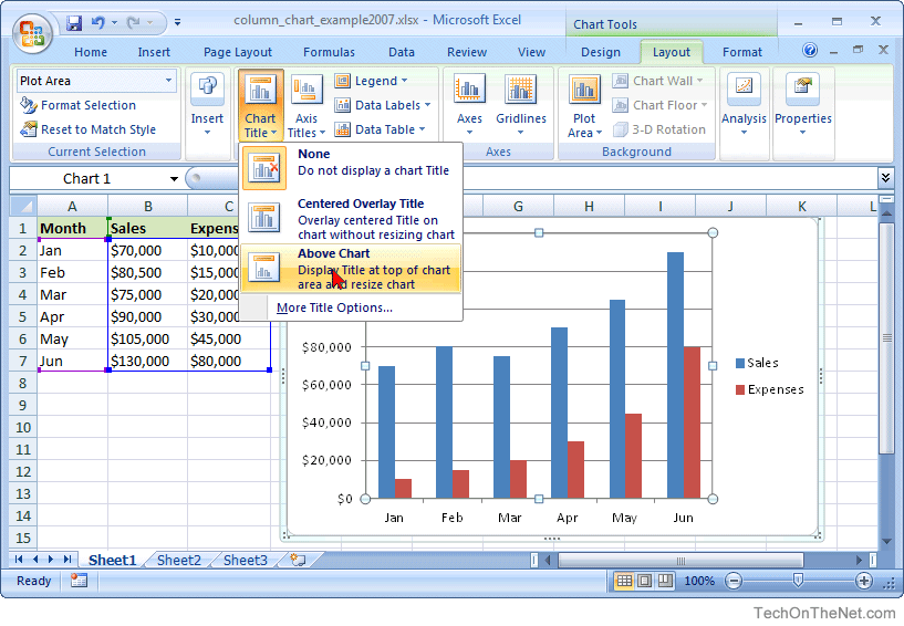
MS Excel 2007: How to Create a Column Chart
Excel Charts - Aesthetic Data Labels - tutorialspoint.com Data Label Positions. To place the data labels in the chart, follow the steps given below. Step 1 − Click the chart and then click chart elements. Step 2 − Select Data Labels. Click to see the options available for placing the data labels. Step 3 − Click Center to place the data labels at the center of the bubbles.

Excel Chart Not Showing All Data Labels - Chart Walls
How to Make a Bar Chart in Excel | Smartsheet Jan 25, 2018 · A data table displays the spreadsheet data that was used to create the chart beneath the bar chart. This shows the same data as data labels, so use one or the other. To add a data table, click the Chart Layout tab, click Data Table, and choose your option. If the legend key option is chosen, you can remove the legend as demonstrated in the ...

How to Change Excel Chart Data Labels to Custom Values?
How to Insert Axis Labels In An Excel Chart | Excelchat Figure 5 – How to change horizontal axis labels in Excel . How to add vertical axis labels in Excel 2016/2013. We will again click on the chart to turn on the Chart Design tab . We will go to Chart Design and select Add Chart Element; Figure 6 – Insert axis labels in Excel . In the drop-down menu, we will click on Axis Titles, and ...

Pie Chart - PK: An Excel Expert
How to Rename a Data Series in Microsoft Excel - How-To Geek To begin renaming your data series, select one from the list and then click the "Edit" button. In the "Edit Series" box, you can begin to rename your data series labels. By default, Excel will use the column or row label, using the cell reference to determine this. Replace the cell reference with a static name of your choice.
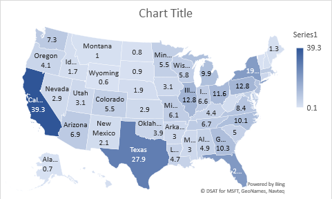
Excel map chart
Prevent Overlapping Data Labels in Excel Charts - Peltier Tech May 24, 2021 · Overlapping Data Labels. Data labels are terribly tedious to apply to slope charts, since these labels have to be positioned to the left of the first point and to the right of the last point of each series. This means the labels have to be tediously selected one by one, even to apply “standard” alignments.

Excel Solution - How to Create Custom Data Label in Chart.avi - YouTube
How do I replicate an Excel chart but change the data? Oct 18, 2018 · To update the data range, double click on the chart, and choose Change Date Range from the Mekko Graphics ribbon. Select your new data range and click OK in the floating Chart Data dialog box. Your data can be in the same worksheet as the chart, as shown in the example below, or in a different worksheet.

Format Number Options for Chart Data Labels in PowerPoint 2011 for Mac
How to change chart axis labels' font color and size in Excel? We can easily change all labels' font color and font size in X axis or Y axis in a chart. Just click to select the axis you will change all labels' font color and size in the chart, and then type a font size into the Font Size box, click the Font color button and specify a font color from the drop down list in the Font group on the Home tab. See below screen shot:
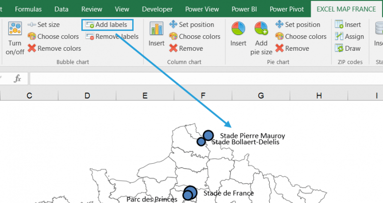
How to geocode customer addresses and show them on an Excel bubble chart? – Maps for Excel ...
Move data labels - support.microsoft.com Click any data label once to select all of them, or double-click a specific data label you want to move. Right-click the selection > Chart Elements > Data Labels arrow, and select the placement option you want. Different options are available for different chart types.
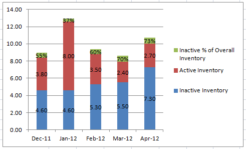
How-to Put Percentage Labels on Top of a Stacked Column Chart - Excel Dashboard Templates
How to Edit Pie Chart in Excel (All Possible Modifications) How to Edit Pie Chart in Excel 1. Change Chart Color 2. Change Background Color 3. Change Font of Pie Chart 4. Change Chart Border 5. Resize Pie Chart 6. Change Chart Title Position 7. Change Data Labels Position 8. Show Percentage on Data Labels 9. Change Pie Chart's Legend Position 10. Edit Pie Chart Using Switch Row/Column Button 11.
Create Charts in Excel - Easy Excel Tutorial
How to add or move data labels in Excel chart? - ExtendOffice In Excel 2013 or 2016. 1. Click the chart to show the Chart Elements button . 2. Then click the Chart Elements, and check Data Labels, then you can click the arrow to choose an option about the data labels in the sub menu. See screenshot: In Excel 2010 or 2007. 1. click on the chart to show the Layout tab in the Chart Tools group. See ...
Creating a chart with dynamic labels - Microsoft Excel 2013
Change axis labels in a chart - support.microsoft.com In a chart you create, axis labels are shown below the horizontal (category, or "X") axis, next to the vertical (value, or "Y") axis, and next to the depth axis (in a 3-D chart).Your chart uses text from its source data for these axis labels. Don't confuse the horizontal axis labels—Qtr 1, Qtr 2, Qtr 3, and Qtr 4, as shown below, with the legend labels below them—East Asia Sales 2009 and ...

Charting in Excel - Adding Data Labels - YouTube
Change the format of data labels in a chart To get there, after adding your data labels, select the data label to format, and then click Chart Elements > Data Labels > More Options. To go to the appropriate area, click one of the four icons ( Fill & Line, Effects, Size & Properties ( Layout & Properties in Outlook or Word), or Label Options) shown here.
Chart's Data Series in Excel - Easy Excel Tutorial
Custom Chart Data Labels In Excel With Formulas Select the chart label you want to change. In the formula-bar hit = (equals), select the cell reference containing your chart label's data. In this case, the first label is in cell E2. Finally, repeat for all your chart laebls. If you are looking for a way to add custom data labels on your Excel chart, then this blog post is perfect for you.

E-xcel Tuts: Add Data Labels to Excel Charts
Add or remove data labels in a chart - support.microsoft.com Click the data series or chart. To label one data point, after clicking the series, click that data point. In the upper right corner, next to the chart, click Add Chart Element > Data Labels. To change the location, click the arrow, and choose an option. If you want to show your data label inside a text bubble shape, click Data Callout.

How-to Use Data Labels from a Range in an Excel Chart - Excel Dashboard Templates
How to Change Excel Chart Data Labels to Custom Values? - Chandoo.org May 05, 2010 · Now, click on any data label. This will select “all” data labels. Now click once again. At this point excel will select only one data label. Go to Formula bar, press = and point to the cell where the data label for that chart data point is defined. Repeat the process for all other data labels, one after another. See the screencast.
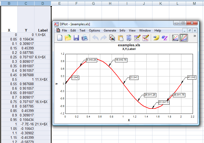
Transferring data > Using the DPlot Interface Add-In for Microsoft Excel > X,Y,Label command
Excel VBA Chart Data Label Font Color in 4 Easy Steps (+ Example) Step 1: Refer to Chart. Refer to the chart with the data label (s) whose font color you want to set. In other words: Create a VBA expression that returns a Chart object representing the applicable chart (with the data label (s) whose font color you want to set). The chart you work with can be either of the following:

Excel Chart Elements and Chart wizard Tutorials
Post a Comment for "44 change data labels in excel chart"