43 how to add data labels to a 3d pie chart in excel

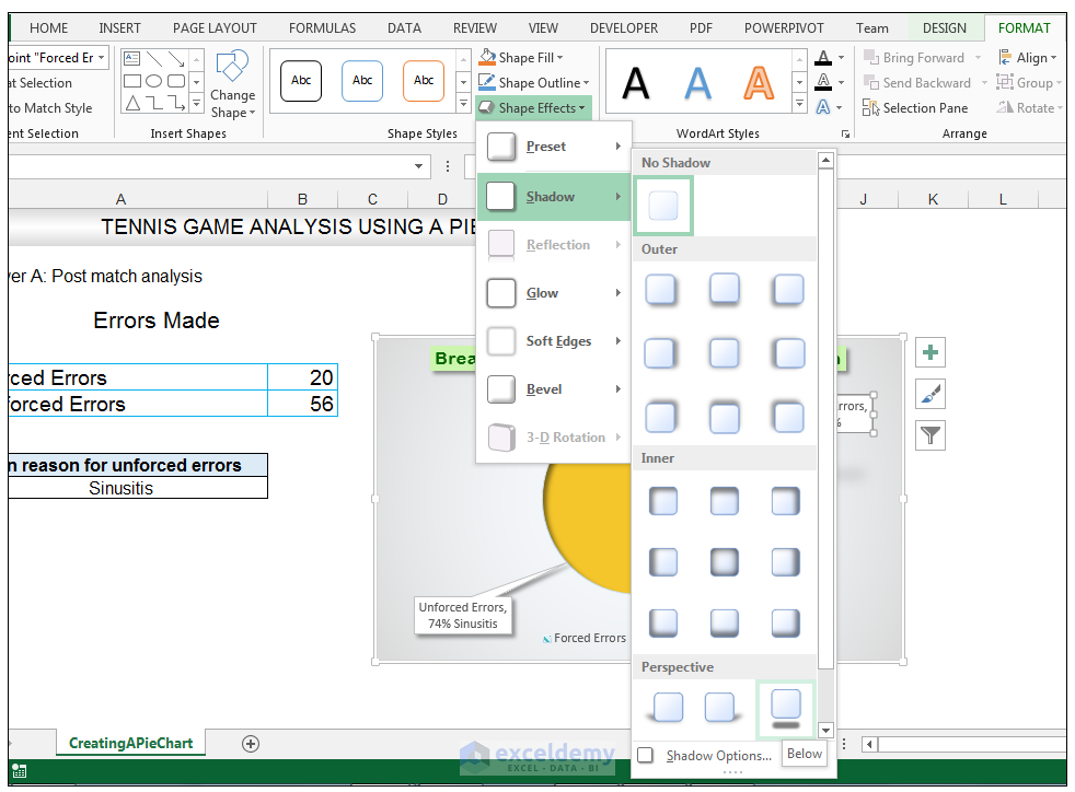
How to Make a Pie Chart in Excel - WinBuzzer Click on your pie chart in Excel and choose a style from the "Chart Design" tab You'll find various styles above the "Chart Styles" heading which will give your chart a fresh look. Press "Change... How to Make a Pie Chart in Excel & Add Rich Data Labels to The Chart! 7) With the data point still selected, go to Chart Tools>Format>Shape Styles and click on the drop-down arrow next to Shape Effects and select Shadow and choose Inner Shadow>Inside Diagonal Top Left. 8) With the one data point still selected, right-click this data point, and select Add Data Label>Add Data Callout as shown below.

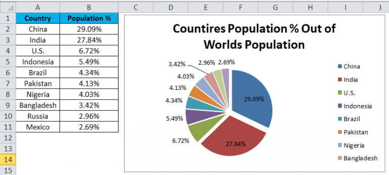
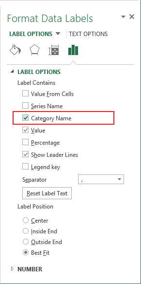
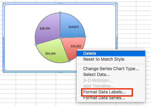
How to Make a Pie Chart with Multiple Data in Excel (2 Ways) - ExcelDemy First, to add Data Labels, click on the Plus sign as marked in the following picture. After that, check the box of Data Labels. At this stage, you will be able to see that all of your data has labels now. Next, right-click on any of the labels and select Format Data Labels. After that, a new dialogue box named Format Data Labels will pop up.

How to add data labels to a 3d pie chart in excel

› ms-excel-pie-chartHow to Make a Pie Chart in Excel (Only Guide You Need) Jul 13, 2022 · Read More: How to Make Pie Chart in Excel with Subcategories (2 Quick Methods) Conclusion. Hope after reading this article you will not face any difficulties with the pie chart. This article covers all the necessary things regarding Excel Pie Chart. Stay tuned for more useful articles. Let us know what problems do you face with Excel Pie Chart. How to add data labels from different column in an Excel chart? This method will guide you to manually add a data label from a cell of different column at a time in an Excel chart. 1. Right click the data series in the chart, and select Add Data Labels > Add Data Labels from the context menu to add data labels. 2. Click any data label to select all data labels, and then click the specified data label to select it only in the chart. Display data point labels outside a pie chart in a paginated report ... Create a pie chart and display the data labels. Open the Properties pane. On the design surface, click on the pie itself to display the Category properties in the Properties pane. Expand the CustomAttributes node. A list of attributes for the pie chart is displayed. Set the PieLabelStyle property to Outside. Set the PieLineColor property to Black.

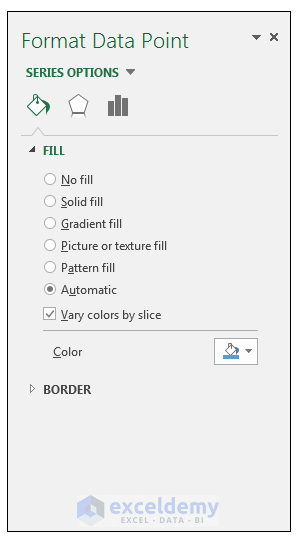
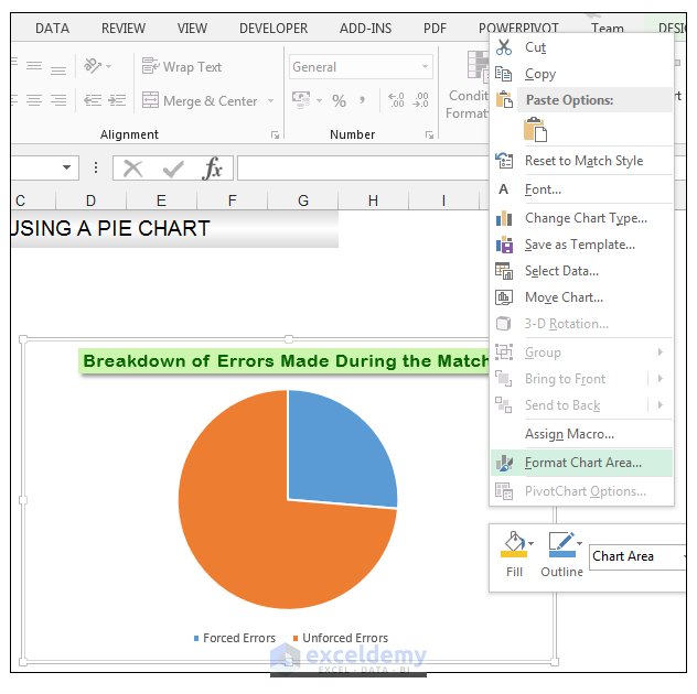
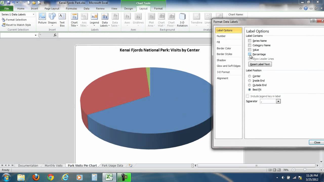
How to add data labels to a 3d pie chart in excel. How to show percentage in pie chart in Excel? - ExtendOffice 1. Select the data you will create a pie chart based on, click Insert > Insert Pie or Doughnut Chart > Pie. See screenshot: 2. Then a pie chart is created. Right click the pie chart and select Add Data Labels from the context menu. 3. Now the corresponding values are displayed in the pie slices. Right click the pie chart again and select Format Data Labels from the right-clicking menu. 4. Excel 2010 data labels not showing on 3d pie chart Every time I open either file and go to the pie chart, only one of the data labels relating to these category's is visible, usually for the section at the top of the chart. If I right click on that one, the others show as empty, highlighted boxes. If I then click on 'format data label' from the drop down list, and either select or de-select ... Excel 3-D Pie charts - Microsoft Excel 2016 - OfficeToolTips On the Insert tab, in the Charts group, choose the Pie button: Choose 3-D Pie. 3. Right-click in the chart area, then select Add Data Labels and click Add Data Labels in the popup menu: 4. Click in one of the labels to select all of them, then right-click and select Format Data Labels... in the popup menu: 5. how to create a line chart in Excel — storytelling with data Insert a line chart. To begin, highlight the data table, including the column headers. To do this, click cell B7 and drag your cursor to C18. Next, navigate to the Insert ribbon and select the line chart icon. (Note that you can also use the Insert menu at the very top, then choose Chart -> Line to achieve a similar result.)

how to add data labels into Excel graphs - storytelling with data To adjust the number formatting, navigate back to the Format Data Label menu and scroll to the Number section at the bottom. I'll choose Number in the Category drop-down and change Decimal places to 0 (side note: checking the Linked to source box is a good option if you want the labels to reformat when the formatting of the underlying source data changes). How To Create A Pie Chart In Excel - PieProNation.com Easy. Either click Add Chart Element from the Chart Layouts command group to the far left of the Design tab or click the green Chart Elements icon next to the chart when its image is selected. To customize data labels, right-click the pie itself and click Format Data Labels from the menu. How to make a 3D pie chart in Excel - Quora Right-click in the chart area, then select Add Data Labels and click Add Data Labels in the popup menu: Click in one of the labels to select all of them, then right-click and select Format Data Labels. Sponsored by SiriusXM I've never tried SiriusXM - what makes it so good? Joe Kolp Edit titles or data labels in a chart - support.microsoft.com On a chart, click one time or two times on the data label that you want to link to a corresponding worksheet cell. The first click selects the data labels for the whole data series, and the second click selects the individual data label. Right-click the data label, and then click Format Data Label or Format Data Labels.

Excel 3-D Pie charts - Microsoft Excel 365 - OfficeToolTips On the Insert tab, in the Charts group, choose the Pie button: Choose the 3-D Pie chart. 3. Right-click in the chart area, then select Add Data Labels and click Add Data Labels in the popup menu: 4. Click in one of the labels to select all of them, then right-click and select Format Data Labels... in the popup menu. 5. Pie Chart in Excel | How to Create Pie Chart - EDUCBA Step 1: Select the data to go to Insert, click on PIE, and select 3-D pie chart. Step 2: Now, it instantly creates the 3-D pie chart for you. Step 3: Right-click on the pie and select Add Data Labels. This will add all the values we are showing on the slices of the pie. How to Create and Format a Pie Chart in Excel - Lifewire To add data labels to a pie chart: Select the plot area of the pie chart. Right-click the chart. Select Add Data Labels . Select Add Data Labels. In this example, the sales for each cookie is added to the slices of the pie chart. Change Colors 3D Plot in Excel | How to Plot 3D Graphs in Excel? - EDUCBA We can add data labels here. Let's plot another 3D graph in the same data. For that, select the data and go to the Insert menu; under the Charts section, select Line or Area Chart as shown below. After that, we will get the drop-down list of Line graphs as shown below. From there, select the 3D Line chart.

How to Make a Pie Chart in Excel & Add Rich Data Labels to The Chart!

› pulse › how-add-total-stackedHow to add a total to a stacked column or bar chart in ... Sep 07, 2017 · The method used to add the totals to the top of each column is to add an extra data series with the totals as the values. Change the graph type of this series to a line graph.

Lesson 38 - How to add DATA LABELS to charts in Excel | Change colour of pie-chart segments in ...

2D & 3D Pie Chart in Excel - Tech Funda To create 2-D Pie chart in Excel, first select the Chart data and go to INSERT menu and click on 'Insert Pie or Doughnut Chart' command dropdown under Charting group on the ribbon. You will see a Pie chart appearing on the page as displayed in the picture below. Notice that Pie chart can only show one type of data (In this case either Actual or ...

Free Pie Chart Maker - Make Your Own Pie Chart | Visme

› legends-in-chartHow To Add and Remove Legends In Excel Chart? - EDUCBA A Legend is a representation of legend keys or entries on the plotted area of a chart or graph, which are linked to the data table of the chart or graph. By default, it may show on the bottom or right side of the chart. The data in a chart is organized with a combination of Series and Categories. Select the chart and choose filter then you will ...

Pie Chart in Excel | How to Create Pie Chart | Step-by-Step Guide Chart

How to Add Data Labels to an Excel 2010 Chart - dummies On the Chart Tools Layout tab, click Data Labels→More Data Label Options. The Format Data Labels dialog box appears. You can use the options on the Label Options, Number, Fill, Border Color, Border Styles, Shadow, Glow and Soft Edges, 3-D Format, and Alignment tabs to customize the appearance and position of the data labels.

Formatting data labels and printing pie charts on Excel for Mac 2019 - - Microsoft Community

› how-to-show-percentage-inHow to Show Percentage in Pie Chart in Excel? - GeeksforGeeks Jun 29, 2021 · Select a 2-D pie chart from the drop-down. A pie chart will be built. Select -> Insert -> Doughnut or Pie Chart -> 2-D Pie. Initially, the pie chart will not have any data labels in it. To add data labels, select the chart and then click on the “+” button in the top right corner of the pie chart and check the Data Labels button.

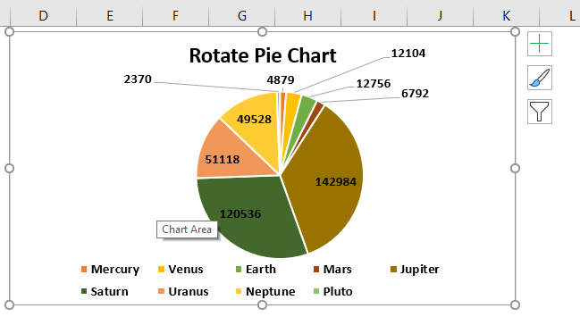
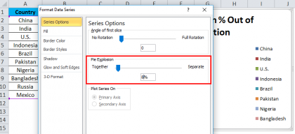
Rotate Pie Chart in Excel | How to Rotate Pie Chart in Excel?

Pie Charts in Excel - How to Make with Step by Step Examples Therefore, the data labels automatically update with a change in the data points. Step 5: Right-click the pie chart again. Click the arrow of "add data labels" and select "add data callouts." The data callouts have been added in the following image. Notice that each slice shows the name of the flavor along with its share in the entire pie.

Excel Tutorials for Beginners

Excel charts: add title, customize chart axis, legend and data labels Select the chart and go to the Chart Tools tabs ( Design and Format) on the Excel ribbon. Right-click the chart element you would like to customize, and choose the corresponding item from the context menu. Use the chart customization buttons that appear in the top right corner of your Excel graph when you click on it.

How to Make a Pie Chart in Excel & Add Rich Data Labels to The Chart!

› pie-chart-examplesPie Chart Examples | Types of Pie Charts in Excel with Examples It is similar to Pie of the pie chart, but the only difference is that instead of a sub pie chart, a sub bar chart will be created. With this, we have completed all the 2D charts, and now we will create a 3D Pie chart. 4. 3D PIE Chart. A 3D pie chart is similar to PIE, but it has depth in addition to length and breadth.

Create Outstanding Pie Charts in Excel | Pryor Learning Solutions

Create a Pie Chart in Excel (In Easy Steps) - Excel Easy Select the pie chart. 9. Click the + button on the right side of the chart and click the check box next to Data Labels. 10. Click the paintbrush icon on the right side of the chart and change the color scheme of the pie chart. Result: 11. Right click the pie chart and click Format Data Labels. 12.

How to Create Excel Pie Charts & Add Rich Data Labels to The Chart!

› plot-multiple-data-sets-onPlot Multiple Data Sets on the Same Chart in Excel Jun 29, 2021 · This will add the secondary axis in the original chart and will separate the two charts. This will result in better visualization for analysis purposes. The combination chart with two data sets is now ready. The secondary axis is for the “Percentage of Students Enrolled” column in the data set as discussed above.

Excel 3-D Pie charts - Microsoft Excel 2013

How to show data labels in charts created via Openpyxl data = Reference (ws, min_col=2, min_row=1, max_col=6, max_row=10) titles = Reference (ws, min_col=1, min_row=2, max_row=10) chart = BarChart3D () chart.add_data (data=data, titles_from_data=True) chart.set_categories (titles) ws.add_chart (chart, "C10") charts label openpyxl Share edited Nov 28, 2019 at 18:31 ozgeneral 5,159 2 23 41

Bar chart | Exceljet

How to Create a Pie Chart in Excel | Smartsheet If want the category names to appear on or near the chart, right-click on the chart and click Add Data Labels …. By default, the numerical values are added. To add other labels, such as the categorical values or the percentage of the total that each category represents, right-click on the chart, then click Format Data Labels ….

Microsoft Excel Tutorials: Add Data Labels to a Pie Chart

r-coder.com › pie-chart-rPIE CHART in R with pie() function [WITH SEVERAL EXAMPLES] An alternative to display percentages on the pie chart is to use the PieChart function of the lessR package, that shows the percentages in the middle of the slices.However, the input of this function has to be a categorical variable (or numeric, if each different value represents a category, as in the example) of a data frame, instead of a numeric vector.

How to Create a Pie Chart in Excel | Smartsheet

How To Make A Pie Chart - PieProNation.com How To Make A Pie Chart In Excel. 1. Create your columns and/or rows of data. Feel free to label each column of data excel will use those labels as titles for your pie chart. Then, highlight the data you want to display in pie chart form. 2. Now, click "Insert" and then click on the "Pie" logo at the top of excel. 3.

Pie Chart in Excel | How to Create Pie Chart | Step-by-Step Guide Chart

How To Create A Pie Chart In Excel With Percentages 3D Pie Chart Adding ... #how #howtocreate #howtocreatepiechart #Piechart #excel #3dpiechart

Creating a 3D Pie Chart in Excel Vid.wmv - YouTube

Add or remove data labels in a chart - support.microsoft.com Click the data series or chart. To label one data point, after clicking the series, click that data point. In the upper right corner, next to the chart, click Add Chart Element > Data Labels. To change the location, click the arrow, and choose an option. If you want to show your data label inside a text bubble shape, click Data Callout.

Excel 3-D Pie Charts

Display data point labels outside a pie chart in a paginated report ... Create a pie chart and display the data labels. Open the Properties pane. On the design surface, click on the pie itself to display the Category properties in the Properties pane. Expand the CustomAttributes node. A list of attributes for the pie chart is displayed. Set the PieLabelStyle property to Outside. Set the PieLineColor property to Black.

Share :