41 excel pivot table conditional formatting row labels

Conditional Format Pivot Table Row | Chandoo.org Excel Forums - Become ... Excel Ninja Apr 3, 2013 #2 Select the entire row, and when you apply the conditional format, make the column reference absolute. So, say we want the entire row 2 to be formatted if cell in col B = 5. formula would be: =$B2=5 Highlighting a row in Pivot Table with Conditional Formatting I suspect it's a pivot table, but can't figure it out. I have a spreadsheet of 1000 + individual rows, with 12 columns. HOWEVER, I'd like to present each row of data in to a little table - so now each row with 12 columns would actually be 12 rows of one column.

Conditional formatting rows in a pivot table ... - MrExcel Message Board What you need to do is accept the formula the way you type it, close the conditional formatting rules manager and then reopen it. Remove the $ from the row numbers that excel added into your formula but leave it on the column number like so =$I3=992, or whatever your first row is.

Excel pivot table conditional formatting row labels

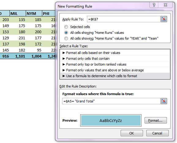
Excel Conditional Formatting in Pivot Table - EDUCBA Click on any cell in the pivot table > Go to the HOME tab > Click on Conditional Formatting option under Styles option > Click on Manage Rules option. It will open a Rules Manager dialog box. Click on the Edit Rule tab, as shown in the below screenshot. It will open the Editing Rule formatting window. Refer to the below screenshot. Design the layout and format of a PivotTable In the PivotTable Options dialog box, click the Layout & Format tab, and then under Layout, select or clear the Merge and center cells with labels check box. Note: You cannot use the Merge Cells check box under the Alignment tab in a PivotTable. Change the display of blank cells, blank lines, and errors conditional formatting per row on pivot - Microsoft Tech Community conditional formatting per row on pivot. I would like to format each row of a pivot table separately (as in the picture shown below), but I cannot paste the formatting. I've got many rows, and they could change (just like the columns) Is there a way to automate this, or I have to select row by row and apply the formatting?

Excel pivot table conditional formatting row labels. Excel Pivot Table Conditional Formatting Row Labels Go making the conditional formatting select the color scale and do it based on commercial and choose diverging and the colors should give expected result. Here a glaze color or bar and been applied... Pivot Table Conditional Formatting for Different Rows Items? Select Your Pivot Table and: Go to Conditional Formatting -> New Rule -> Choose All cells showing "duration" values for "Type and "Date Selection" under "Apply Rule To" section -> Use a Formula to Determine which cells to format and enter the following formula: =AND(A6="Cars",A6>3), You can create new rules for other two conditions as well: Pivot table conditional formatting - Exceljet Select any cell in the data you wish to format and then choose "New rule" from the conditional formatting menu on the Home tab of the ribbon. At the top of the window, you will see setting for which cells to apply conditional formatting to. For the example shown, we want: "All cells showing sum of "sales values" for name and "date" 101 Excel Pivot Tables Examples | MyExcelOnline Jul 31, 2020 · Pivot Tables in Excel are one of the most powerful features within Microsoft Excel. An Excel Pivot Table allows you to analyze more than 1 million rows of data with just a few mouse clicks, show the results in an easy to read table, “pivot”/change the report layout with the ease of dragging fields around, highlight key information to management and include Charts & Slicers for your monthly ...

Conditional Formatting on Pivot Table row labels As per my knowledge, in this case it does not matter what is the source of pivot as after getting the data in pivot, it's the pivot where the conditional formatting need to be applied, please upload a sample. thanks. Regards, DILIPandey DILIPandey +91 9810929744 dilipandey@gmail.com Register To Reply How to remove bold font of pivot table in Excel? - ExtendOffice The normal Bold feature can’t help us to un-bold the row labels in pivot table, but we can apply the powerful function – Conditional Formatting to solve this problem. Please do as follows: 1. Select the bold font row you want to un-bold in the pivot table, or you can press Ctrl key to select multiple bold font rows as your need. See screenshot: Overwrite pivot table conditional format based on row label As far as I know, using the one rule in the Conditional formatting, we can only format the cells with one color if the condition is true and if the same condition is false, the formatting of the cell will be blank and if both conditions are true, the formatting of cell depends on the highest ranking/priority of the rules in Conditional formatting. Apply Conditional Formatting | Excel Pivot Table Tutorial Go to Home Tab → Styles → Conditional Formatting → New Rule. From rule to, select the third option. And, from "select a rule" type select "Format only top or bottom" ranked values. In edit rule description, enter 1 in the input box and from the drop-down menu select "each Column Group". Apply formatting you want. Click OK.

How to Insert a Blank Row in Excel Pivot Table - MyExcelOnline Jan 17, 2021 · STEP 1: Click any cell in the Pivot Table. STEP 2: Go to Design > Blank Rows. STEP 3: You will need to click on the Blank Rows button and select Insert Blank Line After Each Item. NB: For this to work you will need at least two Pivot Table Items in the Rows Labels. You then get the following Pivot Table report: How to Apply Conditional Formatting to Pivot Tables - Excel ... Dec 13, 2018 · How to Setup Conditional Formatting for Pivot Tables. Setting up conditional formatting for pivot tables is a little different than it is for regular cells/ranges. So in this post I explain how to apply conditional formatting for pivot tables. 1. Select a cell in the Values area. The first step is to select a cell in the Values area of the ... Re-Apply Pivot Table Conditional Formatting - yoursumbuddy This method relies on all the conditional formatting you want to re-apply being in that first row labels cell. In cases where the conditional formatting might not apply to the leftmost row label, I've still applied it to that column, but modified the condition to check which column it's in. This function can be modified and called from a ... How to make row labels on same line in pivot table? Make row labels on same line with PivotTable Options You can also go to the PivotTable Options dialog box to set an option to finish this operation. 1. Click any one cell in the pivot table, and right click to choose PivotTable Options, see screenshot: 2.

Re-Apply Pivot Table Conditional Formatting - yoursumbuddy

Excel pivot table conditional formatting row labels Jobs, Ansættelse ... Søg efter jobs der relaterer sig til Excel pivot table conditional formatting row labels, eller ansæt på verdens største freelance-markedsplads med 21m+ jobs. Det er gratis at tilmelde sig og byde på jobs.

How to Apply Data Bars in Pivot Table - MS Excel | Excel In Excel

How to Apply Conditional Formatting to Rows Based on ... - Excel Campus On the Home tab of the Ribbon, select the Conditional Formatting drop-down and click on Manage Rules…. That will bring up the Conditional Formatting Rules Manager window. Click on New Rule. This will open the New Formatting Rule window. Under Select a Rule Type, choose Use a formula to determine which cells to format.

How to Create a MS Excel Pivot Table – An Introduction | SIMPLE TAX INDIA

Excel VBA: Conditional Format of Pivot Table based on Column Label myPivotSourceName = myPivotField.Name. Then rather than referencing the data field with the pivot field object, I referenced the DataRange with the string: myPivotTable.PivotFields (myPivotSourceName).DataRange.Select. Works perfectly and is completely portable for any pivottable on any sheet with any fields. excel vba.

Design your Pivot Table in Excel | Excel in Excel

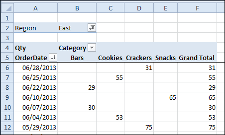
How To Compare Multiple Lists of Names with a Pivot Table Jul 08, 2014 · Column E of the Pivot Table contains the Grand Total (sum of columns B:D). People that volunteered all three years will have a “3” in column E. We should sort the pivot table so all the people with a “3” in column E appear at the top of the list. This will make it easier to find the names.

Sorting a Pivot Table - Free Microsoft Excel Tutorials

101 Advanced Pivot Table Tips And Tricks You Need To Know Apr 25, 2022 · Without a table your range reference will look something like above. In this example, if we were to add data past Row 51 or Column I our pivot table would not include it in the results. To create and name your table. Select your data. Go to the Insert tab and press the Table button in the Tables section, or use the keyboard shortcut Ctrl + T.

What is a Pivot Table in Excel? Everything You Need to Know | Udemy Blog

Conditional Formatting in Pivot Table - WallStreetMojo Currently, a pivot table is blank. Next, we need to bring in the values. Then, drag down the "Date" in the "Rows" Label, "Name" in the "Column," and "Sales" in "Values." As a result, the pivot table will look like the one below. To apply conditional formatting in the pivot table, first, we must select the column to format.

Format Pivot Table Labels Based on Date Range – Excel Pivot Tables

Pivot Table Conditional Formatting Weekend Data Highlight Follow these steps to apply the weekend highlighting in the pivot table: Select all cells where conditional formatting should be applied, cells B5 to B20 in this example. On the Excel Ribbon, click the Home tab. Click Conditional Formatting, and in the drop down menu, click New Rule. The New Formatting Rule dialog box opens.

Share :