41 conditional formatting data labels excel

› charts › progProgress Doughnut Chart with Conditional Formatting in Excel Mar 24, 2017 · Great question! The Excel Web App does not support those text box shapes yet. We can use the built-in data labels for the chart instead. The label for the Remainder bar can be deleted by left clicking on the label twice, then pressing the delete key. That just leaves the data label for the actual progress amount. Here is a screenshot. How to Create Excel Charts (Column or Bar) with Conditional Formatting Conditional formatting is the practice of assigning custom formatting to Excel cells—color, font, etc.—based on the specified criteria (conditions). The feature helps in analyzing data, finding statistically significant values, and identifying patterns within a given dataset.

Progress Doughnut Chart with Conditional Formatting in Excel Mar 24, 2017 · Great question! The Excel Web App does not support those text box shapes yet. We can use the built-in data labels for the chart instead. The label for the Remainder bar can be deleted by left clicking on the label twice, then pressing the delete key. That just leaves the data label for the actual progress amount. Here is a screenshot.

Conditional formatting data labels excel

Conditional Formatting to Distinguish Between Labels and Numbers I want to conditionally format each cell, so that the text is yellow, the numbers are blue, and the blank cells are green. I tried by setting up a new rule under conditional formatting, then selecting "use a formula to determine which cells to format", then using some combinations of the if, istext, isnumber, etc. combinations. Please advise. › pivot-tables › pivot-tableHow to Apply Conditional Formatting to Pivot Tables - Excel ... Dec 13, 2018 · Conditional Formatting can change the font, fill, and border colors of cells. It can also add icons and data bars to the cells. The formatting will also be applied when the values of cells change. This is great for interactive pivot tables where the values might change based on a filter or slicer. How to Setup Conditional Formatting for Pivot ... Custom Conditional Formatting with VLOOKUP? : excel Good evening Excel gurus! Having some trouble with custom formulas for conditional formatting. I have two worksheets, both with two columns, CARDNAME and CARDQUANTITY. The first worksheet is for my COLLECTION, cards I already own, and my second worksheet is for decks I plan to make. (Any MTG players here?)

Conditional formatting data labels excel. How to Apply Conditional Formatting to Rows Based on ... - Excel Campus On the Home tab of the Ribbon, select the Conditional Formatting drop-down and click on Manage Rules…. That will bring up the Conditional Formatting Rules Manager window. Click on New Rule. This will open the New Formatting Rule window. Under Select a Rule Type, choose Use a formula to determine which cells to format. Excel Data Analysis - Conditional Formatting - Tutorials Point Follow the steps to conditionally format cells − Select the range to be conditionally formatted. Click Conditional Formatting in the Styles group under Home tab. Click Highlight Cells Rules from the drop-down menu. Click Greater Than and specify >750. Choose green color. Click Less Than and specify < 500. Choose red color. Conditional format chart data labels | Dashboards & Charts | Excel ... Lance 354 524 550 I create a bar chart that from this data, and display the data label for Actual. I would like to format this data label so that it displays in Red if the value of Actual is less than the value of On Track. Otherwise, it will just display as Blue, which is the format color right now. Changing the Color of a Data Label using IF Statement 1) Click on the data labels to highlight all the data labels, 2) Right-Click and select Format Data Labels, 3) Click on Number, 4) Go to the Format Code field *adapt the following to your needs* 5) [green] [>29]#.00; [<30] [Color 53]#.00 Click to expand... Hi Jawnne, I hope you're still lurking about on here.

Conditional formatting with formulas (10 examples) | Exceljet Here are some examples: = ISODD( A1) = ISNUMBER( A1) = A1 > 100 = AND( A1 > 100, B1 < 50) = OR( F1 = "MN", F1 = "WI") The above formulas all return TRUE or FALSE, so they work perfectly as a trigger for conditional formatting. When conditional formatting is applied to a range of cells, enter cell references with respect to the first row and ... Excel Conditional Formatting not functioning correctly after … Jan 10, 2018 · Everything works fine, formatting changes according to changes in the data! Now I copy a range of sheet A to sheet B using VBA, that works OK. However: in sheet B the conditional formatting of these cells is not working correctly anymore: > cells using 'format only cells that contain' work correct! formatting changes correctly when data changes Conditional formatting based on another column - Power BI Nov 21, 2018 · When I right click on a field and select conditional formatting, the options I have are 'Background color' and 'Font color' whereas all other posts and examples I have seen have 'Background color scales' and 'Font color scales. Within the 'Background color' options I am not able to apply the formatting based on another column as per the link. How to create a chart with conditional formatting in Excel? Add three columns right to the source data as below screenshot shown: (1) Name the first column as >90, type the formula =IF (B2>90,B2,0) in the first blank cell of this column, and then drag the AutoFill Handle to the whole column;

Microsoft Excel conditional number formatting Sep 17, 2019 · Next, I would apply conditional formatting number formatting where the cell value is greater than one so that numbers greater than a million could be displayed to the nearest 0.1m, numbers less than a million but greater than or equal to 1,000 could be displayed to the nearest 0.00k and numbers lower than 1,000 (but necessarily greater than one ... Conditional Formatting with Data Validation - Microsoft Tech Community For example, if A2=Value, B2= Value, and C2 is blank, I would like to have C2 turn red. A2,B2, and C2 all have a list range for the Data Validation. For the conditional formatting, I have only put the range to apply to as column C. The conditional formatting is not turning cells red as needed. I am not sure what the issue is. Excel tutorial: How to add a conditional formatting key That way, we can adjust the conditions for the rules using the key itself. The first step is to create the basic layout for the key. For this, we'll set up a small table with three rows - one for each conditional format. We can then add labels for each conditional format rule. These could be anything, but let's use Excellent, Concern, and ... VBA Conditional Formatting of Charts by Value and Label The first series of the active chart is defined as the series we are formatting. The category labels (XValues) and values (Values) are put into arrays, also for ease of processing. The code then looks at each point's value and label, to determine which cell has the desired formatting. The rows and columns are looped starting at 2, since the ...

Advanced Graphs Using Excel : Gantt Chart in Excel - plot your calender activities

Custom Chart Data Labels In Excel With Formulas Follow the steps below to create the custom data labels. Select the chart label you want to change. In the formula-bar hit = (equals), select the cell reference containing your chart label's data. In this case, the first label is in cell E2. Finally, repeat for all your chart laebls.

Matrix bubble chart with conditional formatting - E90E50fx

Excel Conditional Formatting in Pivot Table - EDUCBA For applying conditional formatting in this pivot table, follow the below steps: Select the cells range for which you want to apply conditional formatting in excel. We have selected the range B5:C14 here. Go to the HOME tab > Click on Conditional Formatting option under Styles > Click on Highlight Cells Rules option > Click on Less Than option.

How to Create Multi-Category Chart in Excel - Excel Board

Format Data Labels in Excel- Instructions - TeachUcomp, Inc. One way to do this is to click the "Format" tab within the "Chart Tools" contextual tab in the Ribbon. Then select the data labels to format from the "Current Selection" button group. Then click the "Format Selection" button that appears below the drop-down menu in the same area.

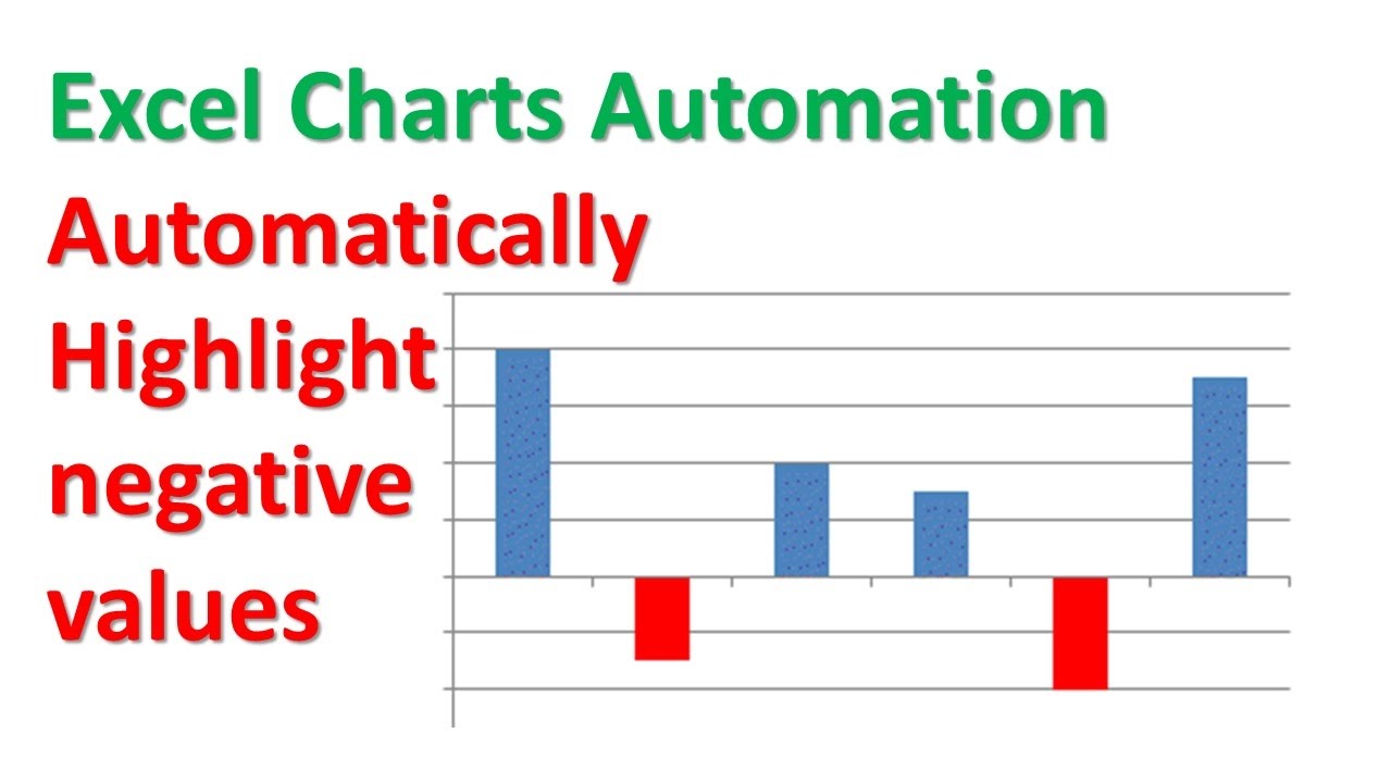
Bar Chart With Negative And Positive Values - Free Table Bar Chart

Creating Conditional Data Labels in Excel Charts - YouTube We can make labels appear on our charts that don't have to do with the raw numbers that built the chart - and we can make them show up or not based on whatever conditions we want. In this tutorial,...

Share :