43 pivot table remove column labels

remove data labels automatically for new columns in pivot chart? I have a query that populates data set for a pivot table. I want data labels to always be at none. Whenever a new column shows up the data label comes back. Anyway I can permanently remove them from the entire pivot chart? this what it looks like when i remove data labels: How to unbold Pivot Table row labels | MrExcel Message Board Under the binocular tab, called FIND AND SELECT, select SELECT OBJECTS. This should place a thin blue line around that and all other subtotals at the same level. Make the changes you want (such as unbolding). P pschommer New Member Joined Nov 18, 2006 Messages 10 Dec 10, 2010 #3 After turning on 'Select Objects', the Font options are grayed out.

How do I hide column headers in pivot table? - FAQ-ANS Hide the Buttons. Right-click a cell in the pivot table and, in the pop up menu, click PivotTable Options. Click the Display tab. In the Display section, remove the check mark from Show Expand/Collapse Buttons. This change will hide the Expand/Collapse buttons to the left of the outer Row Labels and Column Labels .

Pivot table remove column labels

How to Customize Your Excel Pivot Chart Data Labels - dummies To remove the labels, select the None command. If you want to specify what Excel should use for the data label, choose the More Data Labels Options command from the Data Labels menu. Excel displays the Format Data Labels pane. Check the box that corresponds to the bit of pivot table or Excel table information that you want to use as the label. How to Remove Blanks in a Pivot Table in Excel (6 Ways) To find and replace blanks: Click in the worksheet with the pivot table. Click Ctrl + H to display the Replace dialog box. In the Find What box, enter " (blank)". In the Replace with box, type a space if you want to blanks to be removed or type a word such as "Other" to replace the blanks with text. Click Replace Al. How to Move Excel Pivot Table Labels Quick Tricks Use Menu Commands to Move Label. To move a pivot table label to a different position in the list, you can use commands in the right-click menu: Right-click on the label that you want to move. Click the Move command. Click one of the Move subcommands, such as Move [item name] Up. The existing labels shift down, and the moved label takes its new ...

Pivot table remove column labels. How to Remove Duplicates from the Pivot Table - Excel Tutorials Because of this, our Pivot Table is showing two Red colors in column A. When we remove the blank sign and go to our Pivot Table, select it, go to PivotTable Tools >> Analyze >> Refresh, our data will now change: Now we only have one "Red" color in our Spring Color column. Remove Duplicates with Data Formatting How to Control Excel Pivot Table with Field Setting Options Jul 10, 2021 · Quickly Remove a Pivot Field. After you create a pivot table, you might want to remove a field from the layout. You don't need to go to the field list, find that field and remove its check mark, or drag the pivot field out of the Row Labels area in the field list. How to reset a custom pivot table row label Insert a column and make it equal to the Problem column. 4. Now go back to your Pivot and refresh it to find the Problem column and the duplicate column you just made. 5. Enter both fields into the pivot table and you will see the duplicate column has the original values while the Problem column maintains the problem labels. Hide Excel Pivot Table Buttons and Labels Right-click any cell in the pivot table In the pop-up menu, click PivotTable Options In the PivotTable Options dialog box, click the Display tab To hide all of the expand/collapse buttons in the pivot table: Remove the check mark from the option, Show expand/collapse buttons

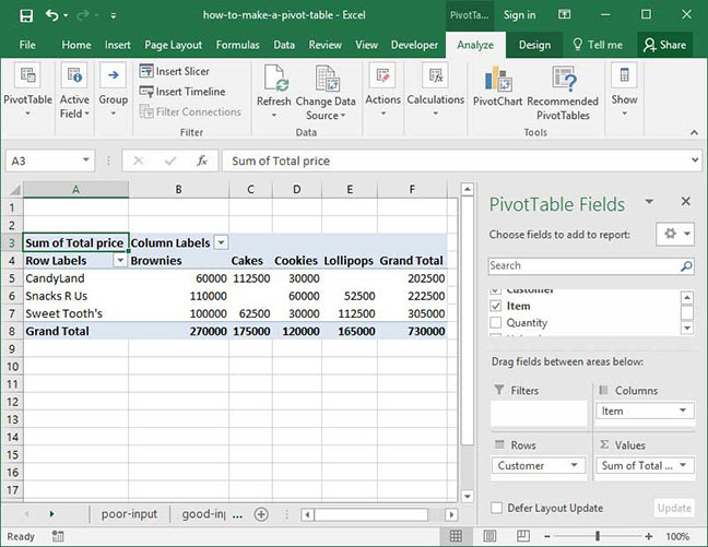
How to delete column label from pivot table field For a new thread (1st post), scroll to Manage Attachments, otherwise scroll down to GO ADVANCED, click, and then scroll down to MANAGE ATTACHMENTS and click again. Now follow the instructions at the top of that screen. New Notice for experts and gurus: How to Use the Excel Pivot Table Field List If this box is not checked, the pivot table is recalculated after each field is added or moved. Turn On Defer Layout Update. To defer the layout updates: Add a check mark to the Defer Layout Update box in the PivotTable Field List. Make Pivot Table Changes. While the Defer Layout Update setting is turned on, make your pivot table changes: Excel pivot table - average of calculated sums - Stack Overflow Add the column to your pivot; Create a formula in your pivot table called Avg per Cust =Value/UniqueCust; This will flag each row in your data with a 1 if it is the first time a name appears in the column or zero otherwise. The pivot table calculation will sum up the total value and divide by the total unique customers. pivot table - Excel PivotTable Remove Column Labels - Super User 1. Good Day, What you are looking to do is hide the row and column headers. Please see the directions below. Click on the View tab. Deselect the heading box. Hope that helps, Brad. Share. Improve this answer.

How to Fix Empty Cells and Error Values in Pivot Table Identify the location of “blank” values in your Pivot Table. In our case, the word “blank” is appearing in Row 8 and also in Column C of the Pivot Table. 2. To hide “blank” values in Pivot Table, click on the Down-arrow located next to “Row Labels”. How to Use Excel Pivot Table Label Filters - Contextures Hide Drop Down Arrow to Prevent Filtering — In an Excel pivot table, you might want to hide one or more of the items in a Row field or Column field. To do ... Automatic Row And Column Pivot Table Labels Select the data set you want to use for your table The first thing to do is put your cursor somewhere in your data list Select the Insert Tab Hit Pivot Table icon Next select Pivot Table option Select a table or range option Select to put your Table on a New Worksheet or on the current one, for this tutorial select the first option Click Ok How to rename group or row labels in Excel PivotTable? 1. Click at the PivotTable, then click Analyze tab and go to the Active Field textbox. 2. Now in the Active Field textbox, the active field name is displayed, you can change it in the textbox. You can change other Row Labels name by clicking the relative fields in the PivotTable, then rename it in the Active Field textbox.

[Solved] Need a step-by-step guide on how to create pivot charts along with the answers to this ...

How to Remove Totals from Pivot Table - Excel Tutorials To do this, we use the same tab as we did above, and go to PivotTable Tools >> Design >> Layout >> Grand Totals. When we click on it, a dropdown menu will appear: As seen, we can remove Grand Totals from rows and columns, we can activate it for both rows and columns, or activate it only for one option.

How To Make A Pivot Table | Deskbright

Clear Old Items in Pivot Table Drop Downs - Contextures Blog Change a Pivot Table Setting. In Excel 2007 or Excel 2010, you can change a pivot table setting, to prevent old items from appearing. Right-click any cell in the pivot table, and click PivotTable options. In the PivotTable Options dialog box, click the Data tab. In the Retain Items section, select None from the drop down list.

Accelerate Your Analysis with Pivot Table | Simplified Excel

Consolidate Pivot Table Column Labels Answers. I have assumed that you have three columns: Date, Doctor, Operation. Select your table and create a pivot table. Then drag Doctor to the Row Field area, Date to the Column Field area, and Operation to the Data Items area TWICE. Choose the second (Operation2), right click it, choose "Field Settings" and select "Show data as % of Row ...

Pivot table row labels in separate columns • AuditExcel.co.za

Removing old Row and Column Items from the Pivot Table Getting rid of old Row and Column Labels from the Pivot Table manually You place yourself in the PivotTable and either Right Click and select PivotTable Options or go to the Analyze (Excel 2013) or Options (Excel 2007 and 2010) Tab. In the PivotTable Options dialog box you place yourself on the Data tab.

How to Create Pivot Table in Excel - All Things How

How to make row labels on same line in pivot table? Please do as follows: 1. Click any cell in your pivot table, and the PivotTable Tools tab will be displayed. 2. Under the PivotTable Tools tab, click Design > Report Layout > Show in Tabular Form, see screenshot: 3. And now, the row labels in the pivot table have been placed side by side at once, see screenshot:

How to Sort Data Manually in the Pivot Table? - MS Excel | Excel In Excel

Hide Pivot Table Buttons and Labels - Contextures Blog Follow these steps to hide the buttons: Right-click a cell in the pivot table and, in the pop up menu, click PivotTable Options. Click the Display tab In the Display section, remove the check mark from Show Expand/Collapse Buttons. This change will hide the Expand/Collapse buttons to the left of the outer Row Labels and Column Labels.

Intro to PivotTables - ExcelWriter v8 Docs - OfficeWriter Docs

How to Group Numbers in Pivot Table in Excel You May Also Like the Following Pivot Table Tutorials: How to Group Dates in Pivot Table in Excel. How to Create a Pivot Table in Excel. Preparing Source Data For Pivot Table. How to Refresh Pivot Table in Excel. Using Slicers in Excel Pivot Table – A Beginner’s Guide. How to Apply Conditional Formatting in a Pivot Table in Excel.

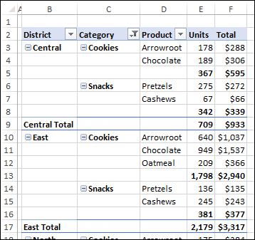
Clean Up Pivot Table Subtotals – Excel Pivot Tables

Remove PivotTable Duplicate Row Labels [SOLVED] The best solution here is to filter that field out in the raw data, select a cell which has the issue, copy and paste it across the column. And for the Vendor Name issue, you can use the same solution. Hope this clarifies.. Regards, Chandra Please click on the 'Add Reputation' button at the bottom of my post if I was helpful in resolving the issue.

How to Sort Pivot Table Row Labels, Column Field Labels and Data Values with Excel VBA Macro ...

How to show multiple grand totals in pivot table? - ExtendOffice Refresh the pivot table by right clicking one cell in the pivot table and choose Refresh, and the new field will be add to the Choose fields to add to report: list box, check and drag the Grand Total field to the Row Labels list box, and put it at top. See screenshot: 3. And a new field blank label will be displayed at the top of the pivot ...

GNIIT HELP: Advance Excel - PivotTable Recommendations ~ GNIITHELP

Delete & Clear Pivot Table Cache | MyExcelOnline Jul 05, 2020 · Click Ok three times and Voila it’s done! The old deleted items from the data source are not shown in the Pivot Table’s filter selection anymore. How To Clear Pivot Table Cache Memory. Conclusion. In this tutorial, you have learned how to delete pivot table cache memory and change the default setting of the retain items deleted from the ...

Better Format for Pivot Table Headings – Excel Pivot Tables

Remove Sum Of in Pivot Table Headings - Excel Pivot Tables To use Find and Replace: Select all the captions that you want to change Press Ctrl + H to open the Find and Replace Window In the Find What box, type "Sum of" (do not add a space at the end) Leave the Replace With box empty Click Replace All, to change all the headings. Pivot Table Tools

Using column label as formatting condition in excel pivot table - Stack Overflow

Design the layout and format of a PivotTable - Microsoft Support In the PivotTable Options dialog box, click the Layout & Format tab, and then under Layout, select or clear the Merge and center cells with labels check box. Note: You cannot use the Merge Cells check box under the Alignment tab in a PivotTable. Change the display of blank cells, blank lines, and errors

More Than One Filter on Pivot Table Field - Contextures Blog

python - How can remove a column name/label from a pivot table and ... I have a pivot table using CategoricalDtype so I can get the month names in order. How can I can drop the column name/label "Month" and then move the month abbreviation names to the same level as "Year"? ... .pivot_table (index='Year',columns='Month',values='UpClose',aggfunc=np.sum)) Current output:

31 How To Label Excel Columns - Labels Database 2020

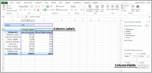
Microsoft Excel - showing field names as headings rather than "Row ... In earlier versions, by default if you create a pivot table, instead of showing the field names, it will say row labels and column labels. To see the field names instead, click on the Pivot Table Tools Design tab, then in the Layout group, click the Report Layout dropdown and select either Show in Outline Form or Show in Tabular form.

How To Manage Big Data With Pivot Tables

How to Remove Old Row and Column Items from the Pivot Table in Excel? Removing Old rows and columns from the Pivot table Given a table students and their marks. A pivot table is also made from the given table. It represents the students and their total marks obtained. Step 1: Deleting the sixth row from the given table i.e. the student name Shubham .

Components | CLEARIFY

Remove row labels from pivot table - AuditExcel Click on the Pivot table Click on the Design tab Click on the report layout button Choose either the Outline Format or the Tabular format If you like the Compact Form but want to remove 'row labels' from the Pivot Table you can also achieve it by Clicking on the Pivot Table Clicking on the Analyse tab

Macro to Repeat Item Labels in Excel Pivot and Flatten

Repeat item labels in a PivotTable - support.microsoft.com Right-click the row or column label you want to repeat, and click Field Settings. Click the Layout & Print tab, and check the Repeat item labels box. Make sure Show item labels in tabular form is selected. Notes: When you edit any of the repeated labels, the changes you make are applied to all other cells with the same label.

Share :